材料初步考察
- 蘑菇书 的形式和编排结构很好, 但数学部分糟糕 (第二章开头就一堆错误, 反正我读不下去).
- Sutton 的经典 Reinforcement Learning: An Introduction 2022 年的第二版. 主要是 value-based, 而非当今流行的 policy-based (书中只有二十几页描述). 没读.
- HuggingFace 也有个 deep-rl-class. 过于简化了而且比较啰嗦, 但是附方便的代码实践.
- OpenAI 的 Spinning Up 简单介绍了 policy gradient.
- CS 285 at UC Berkeley Deep Reinforcement Learning 比较现代. 看了前面一部分. (视频没看, 直接看的 slides.)
- 其他可以参考 Reinforcement Learning Resources — Stable Baselines3.
下面是简要的笔记: 统一了记号, 自己简明的证明和 PyTorch 实现, 还有杂七杂八的补充.
目标
Which algorithms? You should probably start with vanilla policy gradient (also called REINFORCE), DQN, A2C (the synchronous version of A3C), PPO (the variant with the clipped objective), and DDPG, approximately in that order. The simplest versions of all of these can be written in just a few hundred lines of code (ballpark 250-300), and some of them even less (for example, a no-frills version of VPG can be written in about 80 lines). 来自 Spinning Up.
先搞清楚最流行的方法. 至于具体应用场景… 呃… 我没有需求, 就是单纯玩玩而已, 所以不会特别深入, 看多少算多少.
CS 285 Lecture 4: Introduction to Reinforcement Learning
开篇以 top-down 的形式非常清晰地介绍了 RL 的各种算法类型. 记号基本沿用原 slide (有少许改动), 不再全部复读. 其他材料来源的记号也会统一为这个. 很多基本概念不再复读.
补充
- Why was the letter Q chosen in Q-learning? 没有实际意义, 只是原论文在公式中用了这个记号.
- How can I prove that $I-\gamma A$ is invertible?
CS 285 Lecture 5: Policy Gradients
目标是累计收益的期望最大. 累计收益的期望为
\[J(\theta) = \mathbb E_{\tau \sim p_\theta(\tau)} \sum_{t=1}^T r(s_t, a_t),\]其中 $\tau$ 表示 trajectory ($s_1$, $a_1$, $…$, $s_T$, $a_T$).
虽然很多 notes (包括这个) 根本不提数学假设, 但实际需要 **假设可以交换积分和微分** (比如有限离散的时候为有限求和), 为了推导简便也假设期望可以写为良定义的密度函数的积分 (虽然这个假设没必要, 但可以免去麻烦而且不本质的数学细节, 简化符号).下面记 $r(\tau) = \sum_t r(s_t, a_t)$, 用 log-gradient trick
\[\begin{align*} \nabla_\theta J(\theta) = &\int \nabla_\theta p_\theta(\tau) r(\tau) \,\mathrm d\tau \\ = & \int p_\theta(\tau) \nabla_\theta \log p_\theta(\tau) r(\tau) \,\mathrm d\tau \\ = & \mathbb E \nabla_\theta \log p_\theta(\tau) r(\tau) \\ = & \mathbb E \left( \sum_t\nabla_\theta \log \pi_\theta(a_t|s_t) \right) r(\tau), \end{align*}\]最后一步是由 Markov 性.
策略梯度的基本流程就是
- 根据当前的 policy $\pi$ 获得样本 (trajectory)
- 梯度提升 (因为要最大化目标函数) 获得新的 policy, 再重复 step 1
因此原版是 on-policy 的.
Understanding Policy Gradients. 和极大似然相比, 策略梯度的区别是其梯度对 reward 加权了, 高 reward 的 trajectory 会使梯度更多地往那个方向更新.
Off-Policy Policy Gradients. On-policy learning can be extremely (sample) inefficient. 可以用 importance sampling 做 off-policy. In summary, when applying policy gradient in the off-policy setting, we can simple adjust it with a weighted sum and the weight is the ratio of the target policy (the policy we want to learn) to the behavior policy (which is actually acting in the world).
Reducing Variance
为什么方差高?
\[\begin{align*} \nabla_\theta J(\theta) &= \mathbb E \left( \sum_{t=1}^T\nabla_\theta \log \pi_\theta(a_t|s_t) \right) \sum_{t=1}^T r(s_t, a_t) \\ &= \mathbb E \left( \sum_{t=1}^T\nabla_\theta \log \pi_\theta(a_t|s_t) \sum_{t'=t}^T r(s_{t'}, a_{t'}) \right). \end{align*}\]The high variance in vanilla policy gradient arises from the fact that it directly uses the sampled returns to estimate the policy gradient. Since the returns are based on the actual trajectories experienced by the policy, they can have high variability due to the stochastic nature of the environment. This variance can result in noisy gradient estimates, leading to unstable training and slow convergence. 来自 ChatGPT 3.5 的回答.
一开始这里 “reward to go” trick 来自两点, 一是 $\mathbb E \nabla_\theta p_\theta = 0$ (还是一样, 用 log-gradient trick, 交换积分和微分), 二是 Markov 性的一个推论, 过去和未来独立 (可以参考 这里). 所以把独立的两项拆开求期望, 其中一项期望为零, 可以扔掉.
But how is this better? A key problem with policy gradients is how many sample trajectories are needed to get a low-variance sample estimate for them. The formula we started with included terms for reinforcing actions proportional to past rewards, all of which had zero mean, but nonzero variance: as a result, they would just add noise to sample estimates of the policy gradient. By removing them, we reduce the number of sample trajectories needed. 来自 Spinning Up.
为了减少方差, 考虑策略梯度中第二项减去常数 baseline $b$ (不一定常数, 只要和 $\theta$ 无关就行), 即 $\nabla_\theta \log p_\theta(\tau) (r(\tau) - b)$ (因为如上一段所述, 第一项期望为零, 所以这样操作不改变期望). 新式子的方差是关于 $b$ 的二次函数, 求导数为零的点即得最小方差, 可得 $b = \mathbb E g(\tau)^2 r(\tau) / \mathbb E g(\tau)^2$, 其中 $g(\tau) = \nabla_\theta \log p_\theta(\tau)$.
策略梯度这个第二项 (加权方式) 还有很多种选择, 它们期望相同, 但方差不同.
Implementing Policy Gradients
import torch.nn as nn
import torch.nn.functional as F


class PolicyNetwork(nn.Module):
    def __init__(self, state_size, num_actions):
        super().__init__()
        self.fc = nn.Linear(state_size, num_actions)

    def forward(self, state):
        return self.fc(state)


def compute_loss(logits, actions, advantages):
    """
    Parameters:
        logits (torch.Tensor): The output logits from the policy network.
                              Shape: (batch_size, num_actions)
        actions (torch.Tensor): The tensor containing the indices of the actions taken.
                                Shape: (batch_size,)
        advantages (torch.Tensor): The tensor containing the advantages for each time step.
                                   Shape: (batch_size,)
    """
    return F.cross_entropy(logits, actions, weight=advantages)
这里的 advantages 可以看 lecture 6, 只是一种加权方式而已. 另外可以参考 Policy Networks — Stable Baselines3, 很简单.
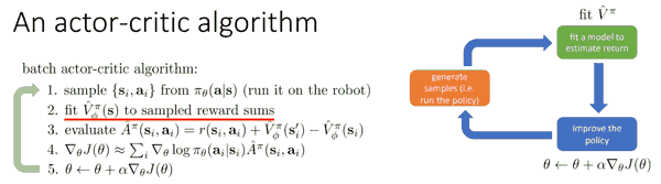
CS 285 Lecture 6: Actor-Critic Algorithms
名字中的 actor 是学习 policy 的东西, critic 则评估收益 (value function).
回到 lecture 5 中 reward-to-go 的式子, 由条件期望的基本性质 (可参考 这里), 注意到
\[\begin{align*} \nabla_\theta J(\theta) &= \mathbb E \left( \sum_{t=1}^T\nabla_\theta \log \pi_\theta(a_t|s_t) \sum_{t'=t}^T r(s_{t'}, a_{t'}) \right) \\ &= \mathbb E \left( \sum_{t=1}^T\nabla_\theta \log \pi_\theta(a_t|s_t) Q(s_{t}, a_{t}) \right), \end{align*}\]其中 $Q(s_{t}, a_{t}) = \sum_{t’=t}^T \mathbb E_{\pi_\theta} (r(s_{t’}, a_{t’}) \mid s_{t}, a_{t})$, cumulative expected reward from taking $a_t$ in $s_t$.
考虑 baseline (value function) $V(s_t) = \mathbb E (Q(s_{t}, a_{t}) \mid s_t) $, 改为用 (advantage) $A(s_{t}, a_{t}) = Q(s_{t}, a_{t}) - V(s_t)$ 替换策略梯度第二项. Advantage 也很容易理解, 就是在给定 state 下这个 action 相比于期望收益的差别.
Value function fitting
注意到 $Q(s_{t}, a_{t}) = r(s_{t}, a_{t}) + \sum_{t’=t+1}^T \mathbb E (r(s_{t’}, a_{t’}) \mid s_{t}, a_{t})$, 下面近似 (去掉积分)
\[A(s_{t}, a_{t}) \approx r(s_{t}, a_{t}) + V(s_{t+1}) - V(s_t),\]因此策略梯度的第二项只需要估计 $V$ 就行. 进一步近似 (去掉积分) $V(s_t) \approx \sum_{t’=t}^T r(s_{t’}, a_{t’})$, 这个可以直接监督学习 (最小二乘) $\left\{ \left( s_{i,t}, \sum_{t’=t}^T r(s_{i,t’}, a_{i,t’}) \right) \right\}$. 进一步, 这里 tuple 的第二项用 $r(s_{i,t}, a_{i,t} + \hat V (s_{i, t+1}) )$, 其中 $\hat V$ 是之前拟合的 value function.
From Evaluation to Actor Critic
以及带 discount 的, 没啥好说的. 后面讨论了加权的变种以及实际实现的变种.
TODO
HuggingFace Unit 2-3: Q-Learning and Deep Q-Learning
HF 的 Q-learning 比 CS 285 讲得明快得多, 对应 Lecture 7: Value Function Methods 和 Lecture 8: Deep RL with Q-Functions.
根据 Markov 性和条件期望基本性质, 易得 Bellman 方程
\[\begin{align*} V(s_t) &= \mathbb E(r(s_t, a_t) \mid s_t) + \sum_{t'=t+1}^T \mathbb E \left( \mathbb E (r(s_{t'}, a_{t'}) \mid s_t, s_{t+1}) \mid s_t \right) \\ &= \mathbb E(r(s_t, a_t) \mid s_t) + \mathbb E (V(s_{t+1}) \mid s_t), \end{align*}\]其中尤其要注意上面的 $V$ 实际依赖 $t$, 只是为了符号简便这样写了 (换种写法, 左边写成 $V_t(s)$, 右边第二项写成 $\mathbb E (V_{t+1}(s’) \mid s)$). 如果有 discount 的话就在第二项前面乘 $\gamma$, 第一项看习惯会简记成 $R_t$ (或者 $R_{t+1}$, 本文取前者). 根据这个就可以动态规划了.
Monte Carlo vs Temporal Difference Learning
In value-based methods, rather than learning the policy, we define the policy by hand and we learn a value function.
Monte Carlo waits until the end of the episode, calculates cumulative return $G_t$ and uses it as a target for updating $V(s_t)$,
\[V^{\mathrm{new}}(s_t) = V(s_t) + \alpha (G_t - V(s_t)),\]where $\alpha$ is the learning rate.
Temporal Difference (TD(0), to be specific) waits for only one interaction (one step $(s_t, a_t, r_t, s_{t+1})$) to form a TD target and update $V(s_t)$. But because we didn’t experience an entire episode, we don’t have $G_t$. Instead, we estimate $G_t$ by $R_t + \gamma V(s_{t+1})$. This is called bootstrapping. It’s called this because TD bases its update in part on an existing estimate $V(s_{t+1})$ and not a complete sample $G_t$.
\[V^{\mathrm{new}}(s_t) = V(s_t) + \alpha (R_t + \gamma V(s_{t+1}) - V(s_t)).\]Q-Learning
Q-Learning is an off-policy value-based method that uses a TD approach to train its action-value function. 是个表格方法, 把所有 state-action pair 对应的 Q-value 都记下来. 因此 state-action pair 数量过大时不适用, 从而引入 deep Q-learning, 输入一个 state, 用神经网络预测每个 action 对应的 Q-value (下一节).
这里 policy 有很多选择, 比如 epsilon-greedy strategy, 就是 $1-\varepsilon$ 的概率选择使 $Q$ 最大的 action, 其他时候探索别的 actions.
而 off-policy 是由于实际与环境交互用 epsilon-greedy strategy, 但是更新 Q 函数时用的 policy 是 greedy strategy.
\[Q^{\mathrm{new}}(s_t, a_t) = Q(s_t, a_t) + \alpha ( r(s_t, a_t) + \gamma \max_a Q(s_{t+1}, a) - Q(s_t, a_t)).\]收敛性的证明见 Convergence of Q-learning: A simple proof. 从上面的表格 Q-iteration 换成非线性的神经网络后, 收敛性不再有保证.
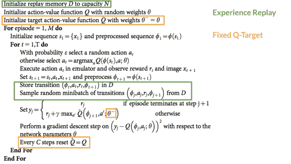
Deep Q-Network (DQN)
The training algorithm has two phases:
- Sampling: we perform actions and store the observed experience tuples in a replay memory.
- Training: Select a small batch of tuples randomly and learn from this batch using a gradient descent update step.
This is not the only difference compared with Q-Learning. Deep Q-Learning training might suffer from instability, mainly because of combining a non-linear Q-value function (Neural Network) and bootstrapping (when we update targets with existing estimates and not an actual complete return).
To help us stabilize the training, we implement three different solutions:
- Experience Replay to make more efficient use of experiences.
- Fixed Q-Target to stabilize the training. 因为不然 estimate 和 target 都依赖同一个参数而且一直变, 就没法优化了.
- Double Deep Q-Learning, to handle the problem of the overestimation of Q-values.
PPO: Proximal Policy Optimization
PPO is a trust region optimization algorithm that uses constraints on the gradient to ensure the update step does not destabilize the learning process. 是的, 就这么简单.
主要 idea 如下. 记 $\theta$ 为旧参数, $\theta’$ 为新参数, 第一个等号的过程略,
\[\begin{align*} J(\theta') - J(\theta) &= \mathbb E_{\tau \sim p_{\theta'}(\tau)} \left( \sum_{t=0}^\infty \gamma^t A^{\pi_\theta}(s_t, a_t) \right) \\ &= \sum_t \mathbb E_{s_t \sim p_{\theta'}(s_t)} [ \mathbb E_{a_t \sim \pi_{\theta'}(a_t \mid s_t)} \gamma^t A^{\pi_\theta}(s_t, a_t) ] \\ &= \sum_t \mathbb E_{s_t \sim p_{\theta'}(s_t)} \left[ \mathbb E_{a_t \sim \pi_{\theta}(a_t \mid s_t)} \frac{\pi_{\theta'}(a_t \mid s_t)}{\pi_{\theta}(a_t \mid s_t)} \gamma^t A^{\pi_\theta}(s_t, a_t) \right]. \end{align*}\]之后想要最外面 $p_{\theta’}$ 也换成 $p_{\theta}$. 然后证明只要 $\pi_{\theta’}(a_t \mid s_t) / \pi_{\theta}(a_t \mid s_t)$ 的绝对值在 1 左右, 则 $p_{\theta’}$ 与 $p_{\theta}$ 也会足够接近, 于是替换后当成新的目标函数来优化. 对于新旧 policy 的约束, PPO 采用了简单的上下界截断, 效果很好而且广为接受.
- Spinning Up guide 注意 PPO is an on-policy algorithm.
CS 285 Lecture 9: Advanced Policy Gradients 的证明来自 Trust Region Policy Optimization (TRPO). 其中推导要成立其实依赖于一些本质的假设 (样本空间有限等), 对于更一般的概率分布是否成立, 我还没空验证, 感觉也不重要了.
补充开头第一个等号的说明. 记号与前面稍有不同, 记 $J(\theta) = \mathbb E_{\tau \sim p_\theta(\tau)} \sum_{t=0}^\infty \gamma^t r(s_t, a_t)$, 则 $V^{\pi_\theta}(s_0) = \mathbb E_{\pi_\theta} (\sum_{t=0}^\infty \gamma^t r(s_t, a_t) \mid s_0)$, 于是
\[\begin{align*} J(\theta') - J(\theta) &= J(\theta') - \mathbb E_{s_0 \sim p(s_0)} V^{\pi_\theta}(s_0) \\ &= J(\theta') - \mathbb E_{\tau \sim p_{\theta'}(\tau)} V^{\pi_\theta}(s_0) \\ &= J(\theta') - \mathbb E_{\tau \sim p_{\theta'}(\tau)} \left[ \sum_{t=0}^\infty \gamma^t V^{\pi_\theta}(s_t) - \sum_{t=1}^\infty \gamma^t V^{\pi_\theta}(s_t) \right] \\ &= J(\theta') + \mathbb E_{\tau \sim p_{\theta'}(\tau)} \left[ \sum_{t=0}^\infty \gamma^t \left( \gamma V^{\pi_\theta}(s_{t+1}) - V^{\pi_\theta}(s_t) \right) \right] \\ &= \mathbb E_{\tau \sim p_{\theta'}(\tau)} \left[ \sum_{t=0}^\infty \gamma^t \left( r(s_t, a_t) + \gamma V^{\pi_\theta}(s_{t+1}) - V^{\pi_\theta}(s_t) \right) \right] \\ &= \mathbb E_{\tau \sim p_{\theta'}(\tau)} \sum_{t=0}^\infty \gamma^t A^{\pi_\theta}(s_t, a_t), \end{align*}\]最后一个等号是由 advantage 函数的定义, 条件期望基本性质, 和 Markov 性.
Hands-on
参考 HF Unit 1 hands-on 改了一些代码.
# https://stackoverflow.com/questions/76222239/pip-install-gymnasiumbox2d-not-working-on-google-colab
swig
gymnasium[box2d]
stable-baselines3[extra]
moviepy  # video
from pathlib import Path

import gymnasium as gym
from stable_baselines3 import PPO
from stable_baselines3.common.env_util import make_vec_env
from stable_baselines3.common.evaluation import evaluate_policy
from stable_baselines3.common.monitor import Monitor
from stable_baselines3.common.vec_env import DummyVecEnv, VecVideoRecorder

env_id = 'LunarLander-v2'
env = make_vec_env(env_id, n_envs=16)

model_path = f'models/ppo-{env_id}'
if Path(model_path + '.zip').exists():
    model = PPO.load(model_path)
else:
    model = PPO(
        policy='MlpPolicy',
        env=env,
        n_steps=1024,
        batch_size=64,
        n_epochs=4,
        gamma=0.999,
        gae_lambda=0.98,
        ent_coef=0.01,
        verbose=1,
        tensorboard_log=f'logs/{env_id}',
    )
    model.learn(total_timesteps=1_000_000)
    model.save(model_path)

eval_env = Monitor(gym.make(env_id))
mean_reward, std_reward = evaluate_policy(
    model=model, env=eval_env, n_eval_episodes=10, deterministic=True,
)
print(f'mean_reward={mean_reward:.2f} +/- {std_reward}')

video_folder = f'videos/{env_id}'
video_length = 300
vec_env = DummyVecEnv([lambda: gym.make(env_id, render_mode='rgb_array')])
vec_env = VecVideoRecorder(
    venv=vec_env,
    video_folder=video_folder,
    record_video_trigger=lambda x: x == 0,
    video_length=video_length,
    name_prefix=f'ppo-{env_id}',
)
obs = vec_env.reset()
for _ in range(video_length + 1):
    action, _ = model.predict(obs)
    obs, _, _, _ = vec_env.step(action)
vec_env.close()
代码封装得很彻底也很简单, 剩下要改的是自定义环境, 一个例子是林亦的 PPO 贪吃蛇 (还有一个更早的其他人的 DQN 贪吃蛇).
几个框架的对比见 这里. 超参数可以参考 rl-baselines3-zoo.
Applications
- ChatGPT: RLHF, GPT-1 到 ChatGPT 简介
- AlphaGo Zero: 基于神经网络的棋类 AI 简介: 以 AlphaGo Zero 和 Stockfish NNUE 为例
- 天风日麻 AI: Suphx
- 星际争霸 AI: AlphaStar
备考
- optuna
- 一文带你理清 DDPG 算法