[半监督] 非监督数据增强 (UDA)

来自 Google 的

Xie, Q., Dai, Z., Hovy, E., Luong, M.-T., & Le, Q. V. (2019). Unsupervised data augmentation for consistency training. arXiv Preprint arXiv:1904.12848. [Code] [Code for PyTorch]

Consistency training methods simply regularize model predictions to be invariant to small noise applied to either input examples or hidden states. This framework makes sense intuitively because a good model should be robust to any small change in an input example or hidden states.

一类半监督学习方法是, 对输入注入扰动后, 使模型依然输出类似的分布, 从而让模型对小扰动不敏感 (类似对抗学习), 对输入空间或者隐空间的变动更平滑. 可以总结如下:

给定输入 $x$, 得到输出分布 $p_\theta (y \mid x)$, 其中 $\theta$ 为模型参数. 给 $x$ 或者 hidden state 加入小扰动 $\varepsilon$ 后, 得到输出分布 $p_\theta(y\mid x, \varepsilon)$.
最小化两个分布之间的 divergence metric (交叉熵, KL 散度, MSE 等) $\mathcal D\left(p_\theta (y \mid x) \;\Vert\; p_\theta(y\mid x, \varepsilon)\right)$.

这里施加的扰动通常是 Gauss 噪声等简单的增强方法.

An early work by Bishop (1995) showed that adding Gaussian perturbation to inputs during the training process is equivalent to adding an extra regularization term to the objective function. (Miyato, et al., 2018)

不同点: UDA 总体结构如下图, 提出用监督学习中的 state-of-the-art 增强方法替换原先的简单增强方法, 包括图中的回译, 图像的随机增强, 以及基于 TF-IDF 的词替换 (替换非关键词) 等.

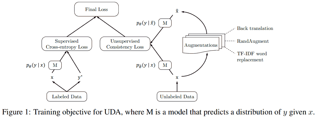
损失函数分为两个部分:

第一部分对于标注数据, 按照通常的方法处理, 其中 $y^\ast$ 表示真实标签, 计算交叉熵.
第二部分对未标注数据, 用原本的参数 $\tilde\theta$ 得到分布预测 $p_{\tilde\theta}(y\mid x)$. 注意这里 $\tilde\theta$ 是 fixed copy of the current parameters $\theta$, 不参与反向传播, 这个 $p_{\tilde\theta}$ 是对真实分布的估计, 在求解优化时固定. 对输入 $x$ 增强得到 $\hat x$, 计算 $p_\theta(y\mid \hat x)$, 计算这两个分布的交叉熵. 因为希望这两个分布相近, 即对于扰动后的样本, 模型输出一致的预测, 这部分称为 consistency loss.

最后把这两个部分加权相加.

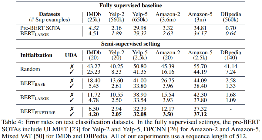
UDA 一个比较惊艳的实验结果是在 IMDb 电影评论分类任务上, 只用 20 个标注数据就达到了不错的效果.

Additional techniques

上述即为核心想法, 除此之外 UDA 在实际实验中使用了一些其他技术.

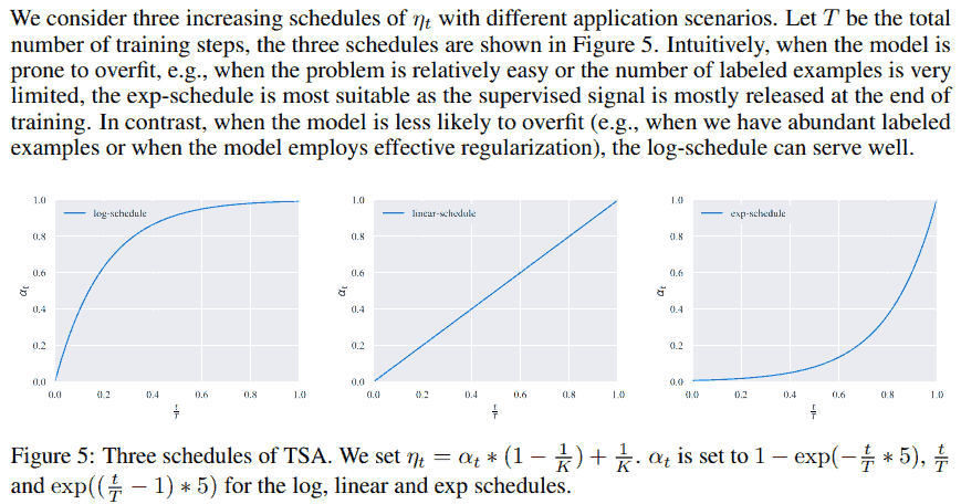
Training signal annealing. Gradually release the “training signals” of the labeled examples as training progresses. 要解决的问题是, 实际中标注数据少, 模型容易在标注数据上快速过拟合, 而在无标注数据上还欠拟合. 想法类似 focal loss, 去掉模型预测得很好的样本, 即如果预测正确的概率大于预先设定的阈值 $\eta_t$, 则不把这个样本对应的 loss 计算进来; 这个阈值随着训练步数 $t$ 的增加逐渐从 $1/K$ 增加到 1, 其中 $K$ 表示类别总数.

下面两个原文是在图像任务上使用的.

Confidence-based masking. 在无标注数据上, 去掉模型不自信的样本. We find it to be helpful to mask out examples that the current model is not confident about. Specifically, in each minibatch, the consistency loss term is computed only on examples whose highest probability among classification categories is greater than a relatively high threshold.

Sharpening predictions. 对无标注数据 Since regularizing the predictions to have low entropy has been shown to be beneficial (Grandvalet and Bengio, 2005; Miyato et al., 2018), we sharpen predictions when computing the target distribution on unlabeled examples by using a low softmax temperature $\tau$ (知识蒸馏用到过的, 文中用了 0.4),

\[p_{\tilde\theta}^{\text{(sharpen)}}(y\mid x) = \frac{\exp(z_y / \tau)}{\sum_{y'} \exp(z_{y'} / \tau)}.\]

Sharpening 和平滑相对, 后者让分布趋向均匀分布, 而前者让突出的更突出 (趋向 one-hot).

Domain-relevance data filtering. We use our baseline model trained on the in-domain data to infer the labels of data in a large out-of-domain dataset and pick out examples that the model is most confident about. Specifically, for each category, we sort all examples based on the classified probabilities of being in that category and select the examples with the highest probabilities.

References

Miyato, T., Maeda, S. I., Koyama, M., & Ishii, S. (2018). Virtual adversarial training: a regularization method for supervised and semi-supervised learning. IEEE transactions on pattern analysis and machine intelligence, 41(8), 1979-1993.
Bishop, C. M. (1995). Training with noise is equivalent to Tikhonov regularization. Neural computation, 7(1), 108-116.
Grandvalet, Y., & Bengio, Y. (2005). Semi-supervised learning by entropy minimization. CAP, 367, 281-296.

Additional techniques

References

Further reading