主要参考
- Hamilton, W. L. (2020). Graph representation learning. Synthesis Lectures on Artifical Intelligence and Machine Learning, 14(3), 1-159.
一本只有 140 页的综述小册子. 本文主要基于第 5-6 章, 简要介绍图神经网络, 不涉及生成式 GNN 等内容.
Aside: 图 (graph) 和网络 (network) 是 “同义词”. 机器学习领域更多用 “图”, 而具体实例更多用 “网络”, 比如社交网络是一个图, 结点表示人, 边表示关系.
Graph neural networks
A key challenge
图神经网络就是在图数据上应用神经网络, 关键是如何生成结点的表示 (node embedding). 通常的深度学习方法不适用于图结构数据, 因为 图没有 “顺序”, 而通常方法的输入是有顺序的 “序列”.
一个朴素的想法是用邻接矩阵作输入. 如果直接把邻接矩阵 $A$ 摊平 (不妨设图有 $n$ 个结点), 输入 MLP (multi-layer perceptron):
\[z = \operatorname{MLP}(A[1] \oplus A[2] \oplus \cdots \oplus A[n]),\]其中 $A[i]$ 表示矩阵 $A$ 的第 $i$ 行向量, $\oplus$ 表示向量拼接. 这种做法的问题是, 输入依赖于结点的顺序: 对结点顺序进行置换 (permutation) 后, 输入表示的图实际没变, 但是网络输出的结果却改变了.
输入邻接矩阵 $A$, 我们希望网络 $f \colon \mathbb R^{n\times n} \to \mathbb R^{n\times m}$ 满足下列性质之一:
\[\begin{align*} &f(PAP') = f(A) \quad &\text{(permutation invariance)},\\ &f(PAP') = Pf(A) \quad &\text{(permutation equivariance)}, \end{align*}\]其中 $P$ 是置换矩阵 (见附录). 第一行置换不变性是说, 当对输入的结点顺序进行置换, 输出应当不变; 第二行置换等变性说, 当对输入的结点顺序进行置换, 输出也应当对应地置换.
Neural message passing
输入图 $\mathcal G = (\mathcal V, \mathcal E)$, 和结点特征 (用来初始化 embeddings) $X \in \mathbb R^{d\times \vert\mathcal V\vert}$, 生成结点 $u$ 的 embedding $z_u$. 其中 $\mathcal V, \mathcal E$ 分别为全体结点集合和全体边集合, $\vert\mathcal V\vert$ 表示集合 $\mathcal V$ 的元素个数. 得到 node embedding 之后, 其他标准的深度学习方法都可以用了.
在 GNN 第 $k$ 次 message-passing 迭代中, 结点 $u$ 的 hidden embedding $h_u^{(k)}$ 根据 $u$ 的邻居 (neighborhood) $\mathcal N(u)$ 中聚合的信息 (也就是标题的 message) 来更新.
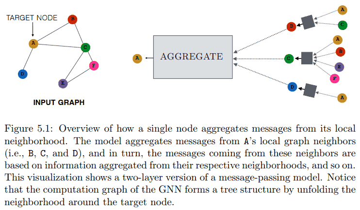
可以表示为
\[h_u^{(k)} = \operatorname{UPDATE}^{(k)}\left( h_u^{(k-1)}, \operatorname{AGGREGATE}^{(k)}(\{ h_v^{(k-1)} : v \in \mathcal N(u) \}) \right).\]初始 embedding 为输入的特征, 即 $h_u^{(0)} = x_u$, 最后一次迭代得到的 hidden embedding 作为 node embedding $z_u$ 输出. 由于 AGGREGATE 的输入为一个集合, 所以如上定义的 GNN 是 permutation equivariant 的. 具体例子, 简单粗暴求和;
\[h_u^{(k)} = \sigma\left( W^{(k)}_{\text{self}} h^{(k-1)}_u + W^{(k)}_{\text{neigh}}\sum_{v\in\mathcal N(u)} h_v^{(k-1)} + b^{(k)} \right).\]为符号简便, 记 $m^{(k)}_{\mathcal N(u)} = \operatorname{AGGREGATE}^{(k)}(\{ h_v^{(k-1)} : v \in \mathcal N(u) \}$. 对这个简单例子,
\[m_{\mathcal N(u)} = \sum_{v\in\mathcal N(u)} h_v.\]显然这个函数 permutation invariant.
Motivations and intuitions
What kind of “information” do these node embeddings actually encode?
结构和特征信息. After the first iteration ($k = 1$), every node embedding contains information from its 1-hop neighborhood, i.e., every node embedding contains information about the features of its immediate graph neighbors, which can be reached by a path of length 1 in the graph; after the second iteration ($k = 2$) every node embedding contains information from its 2-hop neighborhood…
类比 CNN, CNN 关注空间局部信息, GNN 关注结点邻居信息.
Generalized neighborhood aggregation
Neighborhood normalization
对于前面简单粗暴的求和例子, 邻居结点数多的话, 求和会偏大, 导致数值不稳定. 通常办法是除以一个数来标准化, 比如最简单的
\[m_{\mathcal N(u)} = \sum_{v\in\mathcal N(u)} h_v / |\mathcal N(u)|.\]除的数有很多变种, 最流行的基线 GNN——图卷积网络 (GCN)——用了
\[h^{(k)}_u = \sigma \left( W^{(k)} \sum_{v\in\mathcal N(u)\cup {\{u\}}} \frac{h_v}{\sqrt{|\mathcal N(u)| |\mathcal N(v)|}} \right).\]GCN 其实用了一些理论推导出某个东西的近似恰好是上述这样简单的形式, 这个细节不是很重要所以略去.
To normalize or not to normalize? Normalization can lead to a loss of information. For example, after normalization, it can be hard to use the learned embeddings to distinguish between nodes of different degrees. In fact, a basic GNN using the simplest normalization is provably less powerful than the basic sum aggregator. Usually, normalization is most helpful in tasks where node feature information is far more useful than structural information, or where there is a very wide range of node degrees that can lead to instabilities during optimization.
Set aggregators
Janossy pooling is provably more powerful than simply taking a sum or mean of the neighbor embeddings. The idea is to apply a permutation-sensitive function and average the result over many possible permutations.
就是随便找个函数, 然后把结点序列的所有排列组合都输入一遍, 将输出作平均, 再喂给网络. 而由于所有排列组合计算量太大, 实际上通常只随机采样一些排列组合,
Neighborhood attention
加入 attention, 称为 GAT (graph attention network), 比如
\[m_{\mathcal N(u)} = \sum_{v\in\mathcal N(u)} \alpha_{u, v} h_v,\]其中 $\alpha_{u, v}$ 表示 attention.
Generalized update methods
Over-smoothing and neighbourhood influence One common issue with GNNs——which generalized update methods can help to address——is known as over-smoothing. The essential idea of over-smoothing is that after several iterations of GNN message passing, the representations for all the nodes in the graph can become very similar to one another. 这个问题导致 GNN 不能太深.
When we are using a $K$-layer (也就是迭代 $K$ 次) GCN-style model, the influence of node $u$ and node $v$ is proportional the probability of reaching node $v$ on a $K$-step random walk starting from node $u$. An important consequence of this, however, is that as $K \to \infty$, the influence of every node approaches the stationary distribution of random walks over the graph, meaning that local neighborhood information is lost. 细节略.
常见解决办法是 skip connections (此处用向量拼接, 由 GraphSAGE 提出, 当然也有其他方式),
\[\operatorname{UPDATE}_{\text{concat}}(h_u, m_{\mathcal N(u)}) = \operatorname{UPDATE}_{\text{base}}(h_u, m_{\mathcal N(u)}) \oplus h_u.\]剩下的就是把原先 dl 的方法再套一遍, 比如 GRU 等, 略. 得到 node embedding 之后可以基于此得到 graph embedding, 注意 permutation invariance 即可 (比如求和再标准化).
GNN in practice
Applications
三大应用: 结点分类, 图分类, 关系 (边) 预测. 比如预测社交网络中一个用户是不是机器人 (结点分类), 根据分子的图结构预测性质 (图分类), 推荐系统, 知识图谱补全 (关系预测).
随便找了点例子, 主要关注点是如何定义输入的图结构数据.
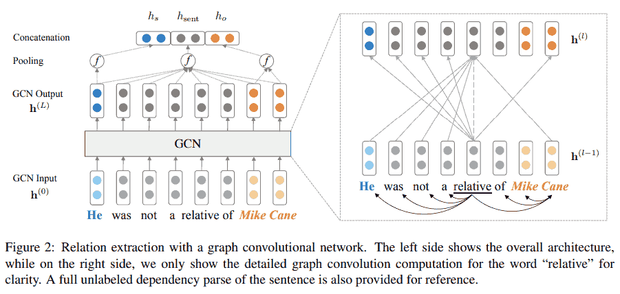
- Zhang, Y., Qi, P., & Manning, C. D. (2018). Graph convolution over pruned dependency trees improves relation extraction. arXiv Preprint arXiv:1809.10185.
这篇是高引文章 (450+引用), 用 GNN + 依存句法进行关系抽取. 但这里所谓的关系抽取其实只是输入主语, 宾语, 和整个句子, 然后预测主语和宾语之间的关系 (分类任务). 输入数据的图结构来自依存关系树, 假设一句话有 $n$ 个 tokens, 记这句话的依存关系树对应的图的邻接矩阵为 $A$, 当第 $i$ 个 token 和第 $j$ 个 token 有依存关系 (图的边) 时, $A_{i, j} = 1$. 模型结构如下, 其中 $h_s$, $h_{\text{sent}}$, $h_o$ 分别表示主语, 句子, 和宾语的 embedding. 除此之外文章还做了一些关于依存关系的优化, 从略.
Efficiency concerns: subsampling and mini-batching
直接对结点进行下采样会遇到的问题是, 会丢失相关联的边的信息, 并且不保证得到的子图还是连通的. 一个策略是转而对结点的邻居采样. 基本想法是, 先选一些结点, 然后递归地采样这些结点的邻居, 同时保证图的连通性. 为了避免采样过多的邻居, 事先设定一个固定数, 只采样这个数量的邻居.
Parameter sharing and regularization
- Parameter sharing across layers The core idea is to use the same parameters in all the AGGREGATE and UPDATE functions in the GNN.
- Edge dropout An essential technique used in the original GAT.
Further reading
- Daigavane, A., Ravindran, B., & Aggarwal, G. (2021). Understanding convolutions on graphs. Distill.
- yyHaker (NewBeeNLP). (2021). 图神经网络从入门到入门.
- 钱雨杰. (2019, Jun 28). 图神经网络如何在自然语言处理中应用?.
- kaiyuan (NewBeeNLP). (2021, May 5). 建议收藏! 早期人类驯服『图神经网络』的珍贵资料.
- 杨晨 (RUC AI Box). (2021, Nov 28). 小白入门: 一文了解推荐系统中的图神经网络.
- 万字综述, GNN 在 NLP 中的应用
工业界实践多用于推荐系统和风控领域. 据一位业务推荐算法工程师分享, GNN 的好处在于泛化好: 很多别的模型可以在小部分曝光上做得很好 (低召回高准确), 但是这对全量来说杯水车薪; 而 GNN 可以帮助泛化到长尾部分 (提高召回), 提高整体效果, 进而拿到更多 item2item 与 user2item 的关系, 持续提升算法效果. 不过大规模 GNN 需要的算力很大 (成百上千节点).
- 黄祥洲. (2021, Dec 20). 图表征学习在美团推荐中的应用.
负面反馈
- Ranger, M. (2021). 2021年的第一盆冷水: 有人说别太把图神经网络当回事儿. [原文]
- 孙天祥. (2021, Apr 10). gnn 正在成为 nlp 领域的鸟粪.
- 王宽. (2021, Oct 29). 精心设计的 GNN 只是 “计数器”?. 微软亚洲研究院.
- 如何评价ACL2022论文用MLP+BoW击败几乎所有基于图的文本分类模型?
- GNN在NLP领域目前能解决哪些BERT不能解决的问题?
苏剑林: 我的视角是没兴趣, 研究都没研究过
TODO
- Bryan Perozzi@Google. Challenges Of Applying Graph Neural Networks
- Pinterest 的落地应用. Graph Convolutional Neural Networks for Web-Scale Recommender Systems
Appendix
Permutation matrix
对 $n$ 个元素的置换 $\pi \colon \{1, \dots, n \} \to \{1, \dots, n \}$ 可以表示为 (Cauchy’s two-line notation)
\[\pi = \begin{pmatrix} 1 & 2 & \cdots & n \\ \pi(1) & \pi (2) & \cdots & \pi(n) \end{pmatrix}.\]用 $e_m$ 表示第 $m$ 个元素为 1, 其余为 0 的行向量, 则 $\pi$ 对应的 $n\times n$ 置换矩阵 $P_\pi$ 可以写为
\[P_\pi = \begin{pmatrix} e_{\pi(1)} \\ e_{\pi(2)} \\ \vdots\\ e_{\pi(n)} \end{pmatrix}.\]易知置换矩阵是正交阵, 且
\[P_\pi^{-1} = P_{\pi^{-1}} = P_\pi'.\]对列向量 $g = (g_1, \dots, g_n)’$, 易知 $P_\pi g = (g_{\pi(1)}, \dots, g_{\pi(n)})’$. 于是可知对矩阵 $M$, $PM$ 置换了 $M$ 的行向量. 类似地, $g’P_\pi = (g_{\pi^{-1}(1)}, \dots, g_{\pi^{-1}(n)})$.
因此对方阵 $A$, 可知 $A_{i, j} = (P_\pi AP’_\pi) _{\pi(i), \pi(j)}$.
- Wikipedia. Permutation matrix.
Graph Laplacian
从 0-1 邻接矩阵 $A$ 可以得到 degree matrix $D$, 它是一个对角阵, 对角线上每个元素代表对应结点的度数, 即 $D_v = \sum A_{v, u}$, Laplace 矩阵则为 $L = D - A$. 对列向量 $x = (x_1, \dots, x_n)’$, 易知 $(Lx)v = L_v x = D_v x_v - \sum{u\in\mathcal N(v)} x_u$, 形如卷积, 只不过不再是邻接空间上的卷积, 而是邻接结点的卷积. 所谓的 Laplace 可以看成五点差分的推广, 即
\[\Delta f(x, y) \approx (f(x+h, y) + f(x-h, y) + f(x, y+h) + f(x, y-h) - 4f(x)) / h^2.\]虽然从 $A$ 变为 $L$ 没有增加任何信息量 (它们是一一对应的), 但是这样的形式更有意义. 还有一种形式是 symmetric normalized Laplacian, 定义为 $D^{-1/2} L D^{-1/2}$, 以及 random walk normalized Laplacian $D^{-1} L$.