回顾经典, 仔细写一下.
原论文
- Lafferty, J., McCallum, A., & Pereira, F. C. (2001). Conditional random fields: Probabilistic models for segmenting and labeling sequence data.
条件随机场 (conditional random field, CRF) 是一种判别式无向概率图模型, 在机器学习中最常见的应用是序列标注.
Markov 性
无向概率图模型又称为 Markov 随机场. Markov 性 通俗地讲即一个随机变量序列 $(Y_1, Y_2, \dots, Y_n)$ 中每个随机变量 $Y_t$ 关于历史序列的条件分布只依赖于前一步 $Y_{t-1}$, 即
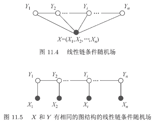
\[\mathbb P(Y_t \in A \mid Y_{t-1}, Y_{t-2}, \dots, Y_1) = \mathbb P(Y_t \in A \mid Y_{t-1}).\] 其中 $A$ 是状态空间对应的 $\sigma$-域的任意集合 (下文省略 $A$).在概率图模型中, 图的每个结点表示一个随机变量 $(Y_v)_{v\in V}$ (其中 $V$ 表示图中所有结点), 边表示随机变量之间的依赖关系. 类似地, 无向图中的 Markov 性指每个随机变量 $Y_v$ 关于其他变量的条件分布只依赖于这个变量的邻居 (直接与它有边连接的所有结点). CRF 中所谓的 conditional 就是全局 conditioned on 另一个随机变量, 即每个结点表示 $Y_v \mid X$ (其中 $X$ 是其他地方来的随机变量, 没有特定的依赖关系):
Let $G=(V, E)$ be a graph such that $Y = (Y_v)_{v\in V}$ so that $Y$ is indexed by the vertices of $G$. Then $(X, Y)$ is a conditional random field when each random variable $Y_v$ conditioned on $X$, obeys the Markov property with respect to the graph; that is, its probability is dependent only its neighbours in $G$:
\[\mathbb P(Y_v \mid X, \{ Y_w: w\ne v \}) = \mathbb P(Y_v \mid X, \{ Y_w: w\sim v \}),\]where $w \sim v$ means that $w$ and $v$ are neighbors in $G$.
从而也能看出 CRF 是判别式模型, 因为其对 $Y \mid X$ 条件分布建模而非对 $(X, Y)$ 联合分布建模.
序列标注
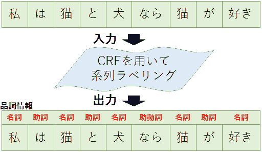
给定一个序列 $x = (x_1, x_2, \dots, x_n)$, 预测每个元素对应的标签 $y = (y_1, y_2, \dots, y_n) \in \mathcal Y^n$. 序列中每个 $x_i$ 表示一个 token (一般为一个字符或者词). 记号 $\mathcal Y$ 表示标签的值域 (如对分词来说一个 token 为一个字符, $\mathcal Y = \{ \text{B}, \text{I}, \text{O} \}$), $\mathcal Y^n$ 表示 $n$ 个 $\mathcal Y$ 的 Descartes 积 $\mathcal Y \times \cdots \times \mathcal Y$.
CRF 结构
一般使用的是特殊的线性链 (linear-chain) CRF (上图两种以及下图最右), 下面讨论的 CRF 都指这种特殊形式. 下面先概述 CRF, 再逐一解释.
特征函数
每个特征函数 (feature function) $f_k(x, t, y_t, y_{t-1})$ 的输入包括
- 序列 $x$
- 当前 token 在序列中的位置 $t$
- 当前 token 的标签 $y_t$
- 前一个 token 的标签 $y_{t-1}$
输出一般为 0 或 1.
例子 (Show more »)
- 若 $y_t$ 为副词且第 $i$ 个词以 "-ly" 结尾, 则返回 1, 否则为 0. 若权重 $\lambda$ 为较大的正数, 说明倾向于把以 "-ly" 结尾的词标注为副词.
- 若 $y_t$ 为动词, $t=1$ 且句子以问号结尾, 则返回 1, 否则为 0. 若权重为较大的正数, 说明 "Is this a sentence beginning with a verb?" 这类句子倾向于把第一个词标注为动词.
- 若 $y_{t-1}$ 为形容词且 $y_t$ 为名词, 则返回 1, 否则为 0.
特征到概率
每个特征函数 $f_k$ 有一个权重 $w_k$, 给定序列 $x = (x_1, x_2, \dots, x_n)$ 和标签 $y = (y_1, y_2, \dots, y_n)$, 定义 score 为
\[\operatorname{score}(y\mid x) = \sum_{k=1}^m\sum_{t=1}^n w_k f_k (x, t, y_t, y_{t-1}),\]其中 $m$ 表示特征函数个数, $n$ 表示序列长度.
将上述 score 用 softmax 归一化得到概率分布
\[p(y \mid x) = \frac{\exp(\operatorname{score}(y\mid x))} {\sum_{l\in \mathcal Y^n}\exp(\operatorname{score}(l\mid x))},\]其中分母一般记为 $Z(x)$. 可以看到 CRF 是个对数线性模型.
训练与预测
CRF 的参数就是 $w = (w_1, \dots, w_m)$, 训练时得到参数估计
\[w^\ast = \underset{w\in \mathbb R^m}{\operatorname{arg max}} \ p_w(y \mid x).\]这个是凸优化, 参数估计不是问题 (比如梯度下降), 深度学习框架自带的优化器即可.
预测时求解概率最大的标注序列,
\[y^\ast = \underset{y \in \mathcal Y^n}{\operatorname{arg max}} \ p_{w^\ast}(y \mid x).\]特征函数的来源
由随机场的基本定理, CRF 的条件概率可写为
\[p(y\mid x) \propto \exp\left( \sum_i\sum_{t=1}^n \lambda_i t_i(x, t, y_t, y_{t-1}) + \sum_j\sum_{t=1}^n \mu_j e_j(x, t, y_t) \right).\]所以 “特征函数” 才能写为上文定义的形式.
很多地方 (包括西瓜书, 李航, 原论文等) 都机械降神般地定义极大团, 然后说由 Hammersley–Clifford 定理, 无向概率图的联合分布可以分解为极大团的表示. 从写机器学习书的角度, 要讲极大团得牵扯到很多概率图模型的内容, 偏离主题而且对其他内容没有帮助, 所以省略掉很合理; 从写论文的角度, 这件事是概率图模型的基本事实 (随机场的基本定理), 也不需要多讲, 给出参考文献即可. 关于引入团 (clique) 的进一步的解释我推荐 PRML p. 385, 该书第 8 章也是很好的概率图模型材料.
一个图模型代表了一个联合分布. 引入图模型的一大用处是便于直观指示随机变量之间的依赖关系, 将联合概率分解成若干条件概率的乘积. 而图模型一大要解决的问题是计算概率 (一堆东西的乘积), 为此需要假设简化结构. 选择线性链 CRF 是因为否则很难计算.与 HMM 对比
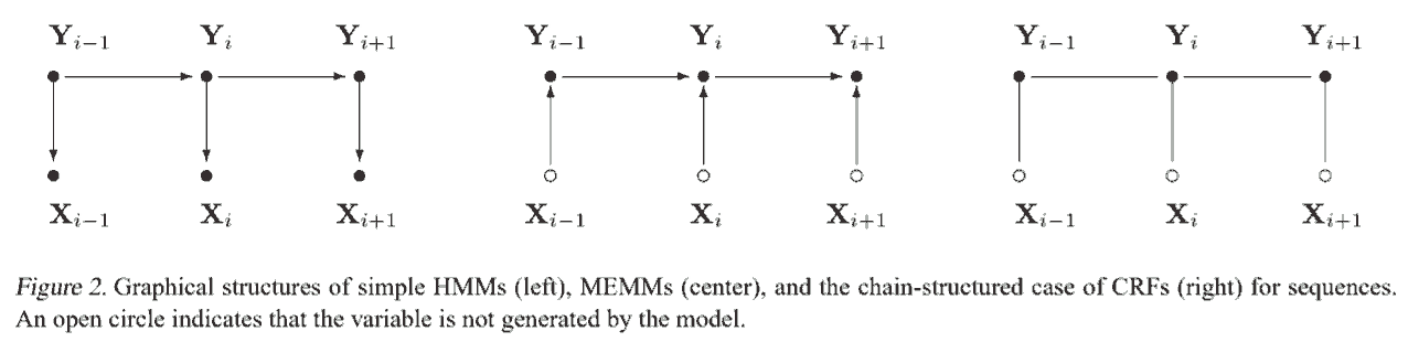
隐 Markov 模型 (hidden Markov model, HMM) 是生成式模型, 假设 $y_t$ 只依赖于 $y_{t-1}$, $x_t$ 只依赖于 $y_t$, 其联合分布为
\[\begin{align*} p(y, x) = p(x \mid y) p(y) \end{align*} = \prod_{t=1}^n \left[p(x_t \mid y_t) p(y_t \mid y_{t-1})\right],\]其中记 $p(y_1) = p(y_1 \mid y_0)$. 上式 $p(x_t \mid y_t)$ 称为发射 (emission) 概率, $p(y_t \mid y_{t-1})$ 称为转移 (transition) 概率. 求对数
\[\log p(y, x) = \sum_{t=1}^n\log p(x_t \mid y_t) + \sum_{t=1}^n\log p(y_t \mid y_{t-1}),\]形式类似 CRF 的 score 函数 (HMM 是 CRF 的子集).
CRF 可以定义大量特征函数 (包括序列全局的特征), 而 HMM 只能处理局部特征.
具体实现
如上述可以定义特征函数的开源实现 (结构如图 11.4) 有 CRF++, 以及 sklearn-crfsuite 等. 把 CRF 作为独立的层实现接在神经网络后面, 一般采用进一步简化的形式 (类比 HMM, 如图 11.5) 如下
\[\log p(y\mid x) = \sum_{t=1}^n \left( T(y_{t-1}, y_t) + E(x_t, y_t) \right) - \log Z(x).\]其中 $T$ 称为 transition score, 可以用 $\vert \mathcal Y \vert \times \vert \mathcal Y \vert$ 的矩阵存储作为 CRF 层的参数 (每个元素为任意浮点数), $E$ 称为 emission score, 一般作为 CRF 层的输入, 由上面的层 (BiLSTM + FC, BERT + FC 等) 给出. 这类的实现数不胜数, 比如 pytorch-crf, 以及 paddlenlp.layers.crf.
计算配分函数
上式第一个求和很容易, 问题在求分母的配分函数 $Z(x)$. 配分函数是 $\vert \mathcal Y \vert^n$ 个 $\exp(…)$ 的求和, 可以用简单的动态规划求解, 以 forward algorithm 为例 (此外还有 backward algorithm 等).
- 初始化: 对任意 $a \in \mathcal Y$, 令
- 对任意 $t=2,\dots,n-1$
- 最后
于是只需要 $n\vert \mathcal Y \vert$ 个 $\exp(…)$ 求和.
Overflow and underflow problem 在 $\log \sum \exp (…)$ 中可能产生浮点数溢出问题. 缓解办法很简单,
\[\log \sum_k \exp (z_k) = \max_i z_i + \log \sum_k \exp( z_k - \max_i z_i).\]框架中有现成的 logsumexp 函数实现.
求解最优标注序列
依然是动态规划 (特别地, 此处叫 Viterbi 算法). 类似 forward algorithm, 迭代时记录每一步 $t$, 起始位置到 $y_t$ 每个可能的标签的最优路径即可.
- 路生. (2022). 如何通俗地讲解 viterbi 算法?
在神经网络中的应用
前面提到 CRF 层的输入为 emission scores, 是由上层网络通过全连接层得到的 (每个 token 一个 $C$ 维向量, 其中 $C$ 表示标签类别总数). 相比于接 softmax ($n$ 个 $C$ 分类), CRF 的作用是增加标签序列之间的依赖关系 (一个 $C^n$ 分类).
CRF 并不是必须的. 比如 BERT 原论文中序列标注就直接用 softmax. 此外还有 sigmoid 预测首尾位置的做法 (指针, 苏剑林不喜欢 CRF 挺喜欢用这种).
另外 CRF 的学习率也需要注意, 苏剑林在 你的 CRF 层的学习率可能不够大 一文中实验发现 BERT 出来的 emission scores 数量级比 CRF 的 transition scores 大了很多, 以至于 CRF 不起作用. 他给出的方案是把 CRF 的学习率调为 BERT 的 100 倍, 让这两个 score 数量级匹配. PaddleNLP 的 CRF 层还专门提供了 crf_lr 参数调节学习率, 并且在官方示例 (examples/information_extraction/waybill_ie) 中接在预训练模型 (Ernie, 类似 BERT) 后时设为了 100.
class ErnieCrfForTokenClassification(nn.Layer):

    def __init__(self, ernie, crf_lr=100):
        super().__init__()
        self.num_classes = ernie.num_classes
        self.crf = LinearChainCrf(
            self.num_classes,
            crf_lr=crf_lr,  # 表示学习率是主体优化器学习率的多少倍
            with_start_stop_tag=False
        )
        ...
与其他概率图模型的对比
vs HMM
与 HMM 对比上面写过了.
生成式模型的缺点 (Show more »)
To define a joint probability over observation and label sequences, a generative model needs to enumerate all possible observation sequences, typically requiring a representation in which observations are task-appropriate atomic entities, such as words or nucleotides. In particular, it is not practical to represent multiple interacting features or long-range dependencies of the observations, since the inference problem for such models is intractable. This difficulty is one of the main motivations for looking at conditional models as an alternative.
A conditional model specifies the probabilities of possible label sequences given an observation sequence. Therefore, it does not expend modeling effort on the observations, which at test time are fixed anyway. Furthermore, the conditional probability of the label sequence can depend on arbitrary, nonindependent features of the observation sequence without forcing the model to account for the distribution of those dependencies. In contrast, generative models must make very strict independence assumptions on the observations, for instance conditional independence given the labels, to achieve tractability.
vs MEMM
最大熵 Markov 模型 (maximum-entropy Markov model, MEMM), 也是判别式模型
\[\begin{align*} p(y\mid x) &= \prod_{t=1}^n p(y_t \mid y_{t-1}, \dots, y_1, x_1, \dots, x_n) \\ &= \prod_{t=1}^n p(y_t \mid y_{t-1}, x_1, \dots, x_n). \end{align*}\]第一个等号是恒等式, 第二个等号来源于模型假设, 就是全局 conditioned on $x$ 之后, $y_t$ 只依赖于 $y_{t-1}$. 类似 CRF,
\[p(y_t\mid y_{t-1}, x) = \frac{\exp(w\cdot f(x, t, y_t, y_{t-1}))} {\sum_{\gamma\in \mathcal Y}\exp(w\cdot f(x, t, \gamma, y_{t-1}))}.\]与 CRF 的不同之处在于分母的处理. CRF 除以所有可能的标注序列 (全局归一化), 而 MEMM 对每一个状态归一化 (per-state normalization). 这就导致了 label bias 的问题 (the transitions leaving a given state compete only against each other, rather than against all other transitions in the model). 原论文第二节讨论了这个问题.
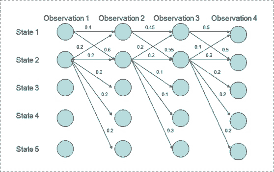
虽然 state 1 转移到 state 2 概率最大, 而且 state 2 保持 state 2 的概率最大, 但是可得最优路径是 state 1 -> 1 -> 1 -> 1. 以为 state 2 可转移的状态比 1 更多, 每个转移选项的概率更小, 而 MEMM 每一步归一化导致它更倾向于选择拥有更少转移状态的 state 1.
不过 MEMM 的优势是训练快.
An advantage of MEMMs versus HMMs and conditional random fields (CRFs) is that training can be considerably more efficient. In HMMs and CRFs, one needs to use some version of the forward–backward algorithm as an inner loop in training. However, in MEMMs, estimating the parameters of the maximum-entropy distributions used for the transition probabilities can be done for each transition distribution in isolation.
为什么叫最大熵? 因为 This form for the distribution corresponds to the maximum entropy probability distribution satisfying the constraint that the empirical expectation for the feature is equal to the expectation given the model. 这个讲起来太长了, 可以参考 wiki.
References
- Marcos Treviso. (2019). Implementing a linear-chain Conditional Random Field (CRF) in PyTorch
- Edwin Chen. (2012). Introduction to Conditional Random Fields
- Michael Collins. Log-Linear Models, MEMMs, and CRFs
Image sources
- 金子冴. (2018).【技術解説】CRF(Conditional Random Fields)
- Scofield. (2019). 解释条件随机场模型