什么是可解释性
可解释性大致想法是理解模型为什么给出当前的预测结果. 但至少我目前没有看到可靠清晰的定义和广泛接受的 benchmark, 故不过多展开. 可以参考
- 要研究深度学习的可解释性, 应从哪几个方面着手? 李 rumor 的回答
- 深度学习的可解释性方向的研究是不是巨坑? ninghaoo 的回答, Akiko 的回答
- 神经网络的可解释性是我们的错觉吗
Side note: 有些地方还会区分 interpretability 和 explainability, 我觉得没什么实际意义.
一些典型方法: 以 TrustAI 为例
通常我们更关心性能 (比如准确率等指标), 寻求可解释性是为了提升性能 (通过分析数据集构造更好的数据集).
Paddle 系列一直是缝合怪, 而且绑定 Paddle 框架, 但是它们包里提到或者实现的方法一般都很经典, 可以作为起步时的参考. 下文主线参考 PaddleNLP 中 applications/text_classification 提到的调优方案针对数据集分析的方法 (Paddle 的 TrustAI).
以文本分类应用为例, 它提供的方案包括
- 稀疏数据筛选: 挖掘稀疏数据 (待预测数据中缺乏证据支持的数据), 之后有选择地增强或补充标注数据.
- 脏数据清洗: 计算训练数据对模型的影响分数, 分数高的样本表明对模型影响大, 可能为脏数据 (标注错误, 去掉或者重标).
- 归因: 样本级别或者 token 级别
这些都是通过对神经网络预测的归因得到的. 下面介绍三个 PaddleNLP 示例中出现的方法 feature similarity, representer point, 以及 integrated gradients.
KNN: feature similarity
trustai.interpretation.FeatureSimilarityModel
最简单直接的样本级别归因.
先得到所有训练样本的 features 向量 (原本网络最后一个全连接层的输入). 对每个预测样本, 根据其 features 查找与其 features top N 相似的训练样本, 作为预测的支持证据.
这里的 features 可以换成梯度等其他向量.
Side note: 从既有网络中取中间值可以通过各种框架的 hook 实现, 比如 PyTorch 的 register_forward_hook.
Paddle 筛选稀疏数据也是通过这个. 验证集和训练集两两求相似度, 如果某个验证集中的数据与它最相似的几个训练样本相似度低则视为稀疏数据.
def get_sparse_data(analysis_result, sparse_num):
    """
    Get sparse data
    """
    idx_scores = {}
    preds = []
    for i in range(len(analysis_result)):
        scores = analysis_result[i].pos_scores
        idx_scores[i] = sum(scores) / len(scores)
        preds.append(analysis_result[i].pred_label)

    idx_socre_list = list(sorted(idx_scores.items(), key=lambda x: x[1]))[:sparse_num]
    ret_idxs, ret_scores = list(zip(*idx_socre_list))
    return ret_idxs, ret_scores, preds
Sample level: representer point
trustai.interpretation.RepresenterPointModels
- Yeh, C. K., Kim, J., Yen, I. E. H., & Ravikumar, P. K. (2018). Representer point selection for explaining deep neural networks. Advances in neural information processing systems, 31. [Github]
文章要点可以参考 ML@CMU 的博客 Representer Point Selection for Explaining Deep Neural Networks.
以多分类任务为例.
原始训练: 输入 -> 原模型全连接层前面网络层 (下称中间层) -> features -> 全连接层 -> logits -> 经过 softmax 变成 probs -> 与真实标签求 loss (交叉熵)
方法一. 只在 loss 加上 L2 正则训练: 输入 -> 原模型全连接层前面网络层 -> features -> 全连接层 -> logits -> probs -> 与真实标签求 loss (交叉熵) + L2 正则
方法二. 如果已经有训练好的模型, 还是 loss + L2, 但只重新训练全连接层: 原模型得到 features -> 全连接层权重根据原模型最后一层初始化 -> 新 logits -> 新 probs -> 把原模型输出的 probs 视为真实标签 求 loss + L2 正则
通过对待 L2 正则的新 loss 求导取驻点 (梯度为零), 可以把最终输出分解成训练集数据 features 的加权平均.

记号
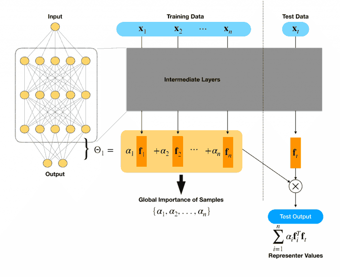
记原始样本 $x_i$ 经过中间层后得到的 feature 为 $m$ 维列向量 $f_i$, 经过全连接层后得到 logits 为 $c$ 维 ($c$ 为多分类类别数量) 列向量 $z_i$, 经过 softmax 后得到概率分布列向量 $p_i$. 记真实标签向量为 $y_i$ ($c$ 维的 0-1 值列向量), 重新训练全连接层后经过 softmax 得到的概率分布为 $q_i$.
文中所谓的对第 $i$ 个样本全局权重 $\alpha_i = -\frac{1}{2\lambda n}\frac{\partial L}{\partial z_i}$, 其中 $n$ 为样本总数, $\lambda$ 为 L2 正则系数, $L$ 为不带正则的原始 loss. 在交叉熵 loss 下, 这个梯度为 $p_i$ - $y_i$ 或者 $q_i$ - $p_i$.
根据上述记号全连接层 (不考虑 bias) 是 $c\times m$ 的矩阵 $A = \sum_{i=1}^n \alpha_i f_i’$. 对任意样本 $x_t$ 得到的 feature $f_t$, 通过全连接层得到的 logits 为 $Af = \sum_{i=1}^n \alpha_i f_i’f_t$, 也就是新样本与每个训练样本的特征求内积相似度 (feature similarity), 然后和对应的权重 (global sample importance) 相乘. 而这个权重就是梯度乘个常数, 对交叉熵损失其梯度就是简单的预测概率与真实概率相减.
文中称 $f_i’f_t$ 是 representer value for $x_i$ given $x_t$, 以及 $\alpha_i f_i’f_t$ 为 representer point.
Intuition for the Representer Theorem and examples of prototypes: For the representer value to be positive, we must have both global sample importance and the feature similarity to have the same sign. For a particular test image, this means that both the test image and training image look similar to each other, and (likely) have the same classification label. Similarly, for this value to be negative, the global sample importance and the feature similarity should have different signs e.g. one is negative and the other is positive. For a particular test image, this means that the images may look similar to each other, but they have different classification labels.
个人疑惑. 上面这段是作者原话, 但是注意 $\alpha$ 正比于 $y-p$ (或者 $p-q$). 为简便起见下面靠考虑二分类 ($y$ 只有一维). 若 $y=1$ 则 $\alpha$ 为正; 若 $y=0$ 则 $\alpha$ 为负. 和上文说的是不是很可能有相同的 label 并没有关系, 意味着这段话是 nonsense.
原作者代码写得很迷, 下面是我写的版本 (Show more »)
import torch
import torch.nn as nn

class Classifier(nn.Module):
    def __init__(self, pretrained_linear: nn.Linear):
        super().__init__()
        assert pretrained_linear.bias is not None  # changeable
        self.linear = nn.Linear(
            in_features=pretrained_linear.in_features,
            out_features=pretrained_linear.out_features,
            bias=True,
        )
        self.linear.weight.data = pretrained_linear.weight.data.clone()
        self.linear.bias.data = pretrained_linear.bias.data.clone()

    def forward(self, x):
        return self.linear(x)


def calculate_alphas(
    classifier: Classifier, features, target_probs,
    learning_rate=1, lambda_=0.003, num_epochs=40000,
    device='cpu',
):
    """
    features (N, m)
    target_probs (N, num_classes)
    alphas (N, num_classes)
    """
    features = torch.Tensor(features).to(device)
    target_probs = torch.Tensor(target_probs).to(device)
    classifier = classifier.to(device)

    # loss_fn = nn.CrossEntropyLoss()  # changeable
    loss_fn = nn.BCEWithLogitsLoss()
    optimizer = torch.optim.SGD(classifier.parameters(), lr=learning_rate)
    min_loss = float('inf')
    min_grad = float('inf')
    patience = 3000
    steps_without_improvement = 0
    best_weights = None

    for epoch in range(num_epochs):
        optimizer.zero_grad()
        l2_norm = torch.sum(
            torch.square(
                torch.cat(
                    [
                        classifier.linear.weight.data,
                        classifier.linear.bias.data.unsqueeze(dim=1),
                    ],
                    axis=1,
                )
            )
        )  # changeable, bias included
        logits = classifier(features)
        loss = loss_fn(logits, target_probs) + lambda_ * l2_norm
        loss.backward()
        optimizer.step()

        grad = torch.cat(
            [
                classifier.linear.weight.grad,
                classifier.linear.bias.grad.unsqueeze(dim=1),
            ],
            axis=1,
        )
        # grad_norm = torch.norm(grad).item()
        grad_norm = torch.mean(torch.abs(grad)).item()
        if grad_norm < min_grad:
            min_grad = grad_norm
            best_weights = classifier.state_dict()

        # TODO: stop criterion
        if loss.item() < min_loss:
            min_loss = loss.item()
            steps_without_improvement = 0
        else:
            steps_without_improvement += 1
            if (steps_without_improvement >= patience) and (min_grad < 1e-6):
                break

        if (epoch + 1) % 100 == 0:
            print(f'Epoch [{epoch + 1}/{num_epochs}], Loss: {loss.item()}, Min Grad: {min_grad}')

    classifier.load_state_dict(best_weights)
    logits = classifier(features)
    # changeable, different derivative for different loss_fn
    # pred_probs = F.softmax(logits, dim=1)
    pred_probs = torch.sigmoid(logits)
    derivative = pred_probs - target_probs
    num_samples = len(features)
    alphas = - derivative / (2.0 * lambda_ * num_samples)
    return alphas
下面再来看看 Paddle 的应用, applications/text_classification/multi_label/analysis/dirty.py. 把对模型影响大的数据视为脏数据取出来. 下面 weight_matrix 就是 $\alpha$.
def get_dirty_data(weight_matrix, dirty_num, threshold=0):
    """
    Get index of dirty data from train data
    """
    scores = []
    for idx in range(weight_matrix.shape[0]):
        weight_sum = 0
        count = 0
        for weight in weight_matrix[idx].numpy():
            if weight > threshold:
                count += 1
                weight_sum += weight
        scores.append((count, weight_sum))
    sorted_scores = sorted(scores)[::-1]
    sorted_idxs = sorted(range(len(scores)), key=lambda idx: scores[idx])[::-1]

    ret_scores = sorted_scores[:dirty_num]
    ret_idxs = sorted_idxs[:dirty_num]

    return ret_idxs, ret_scores
实际上是对每个 sample 算两个值: ($\alpha$ 为正的项的数量, $\alpha$ 为正的项的和). 根据这个排序, 把这两个值最大的前若干个数据视为脏数据. 还是回到上文所述, $\alpha$ 正比于 $y-p$. 所以只拿正值大的数据相当于拿标注为 1 但预测确信为 0 的数据, 好像不太有道理. 拿梯度最大的数据当脏数据还能 make sense, 但这样应该取 $\alpha$ 绝对值最大的数据 (原论文也是这样做的).
Feature level: integrated gradient
trustai.interpretation.IntGradInterpreter
直接看苏剑林的 积分梯度: 一种新颖的神经网络可视化方法.
这类方法的缺陷不是已经被理论证明了吗?好多论文已经否定其可靠性。解释权重对积分路径敏感,路径不唯一,结果就不同,没有一个确切的真理性结果。退一步说,如果穷举积分路径,那跟前人Shapley value就没有区别了。很多类似论文的作者,自己都清楚这些毛病,文章里面浅浅的聊几句,又不点透。。。呵呵了。
其他
- cleanlab: 置信学习.
- Captum: Captum (“comprehension” in Latin) is an open source, extensible library for model interpretability built on PyTorch (同一团队写的). 大多示例用的是积分梯度, 比如 这个 文本分类 token 归因.
- shap (Github): SHAP (SHapley Additive exPlanations) is a game theoretic approach to explain the output of any machine learning model. It connects optimal credit allocation with local explanations using the classic Shapley values from game theory and their related extensions (see papers for details and citations). 特征级别可视化归因.
- LIME
- 2020年了,你还在用注意力作可解释吗?